The Problem
Today we look at problem 5.1 Dodgy Coins, from Ben Lambert’s book A Student’s Guide to Bayesian Statistics.
3 coins, 1 bag:
- Coin 1 is biased towards heads (\(\theta_1 = 0.75\))
- Coin 2 is fair (\(\theta_2 = 0.50\))
- Coin 3 is biased towards tails (\(\theta_3 = 0.25\))
Wanna see a magic trick?
Imagine that we take a coin from the bag and then flip it.
Let:
- \(C = \{1,2,3\}\) denote the identity of the coin (i.e. the outcome of the first experiment)
- \(X = \{T, H\} = \{0,1\}\) denote the outcome of the coin toss
- \(\theta_c\) denote the probability of heads of coin \(C = c\).
Note that \(X\) and \(C\) are random variables and \(\theta_c, \forall c \in C\) is our parameter set (total of 3 parameters).
For a single coin toss \(X = 1\) (heads), we can calculate the probability of getting heads, given the identity of the coin:
\[ Pr(X = 1 \mid C = c) = \theta_c \]
Using the equivalence relation1 we can calculate the likelihood of the coin’s identity given the data:
\[ L(C = c \mid X = 1) = Pr(X = 1 \mid C = c) = \theta_c \]
The sum of the likelihood of all parameter values, in this instance, is hence given by:
\[ \sum_{c = 1}^{3} Pr(X=1 \mid C = c) = \theta_1 + \theta_2 + \theta_3 = 1.5 \]
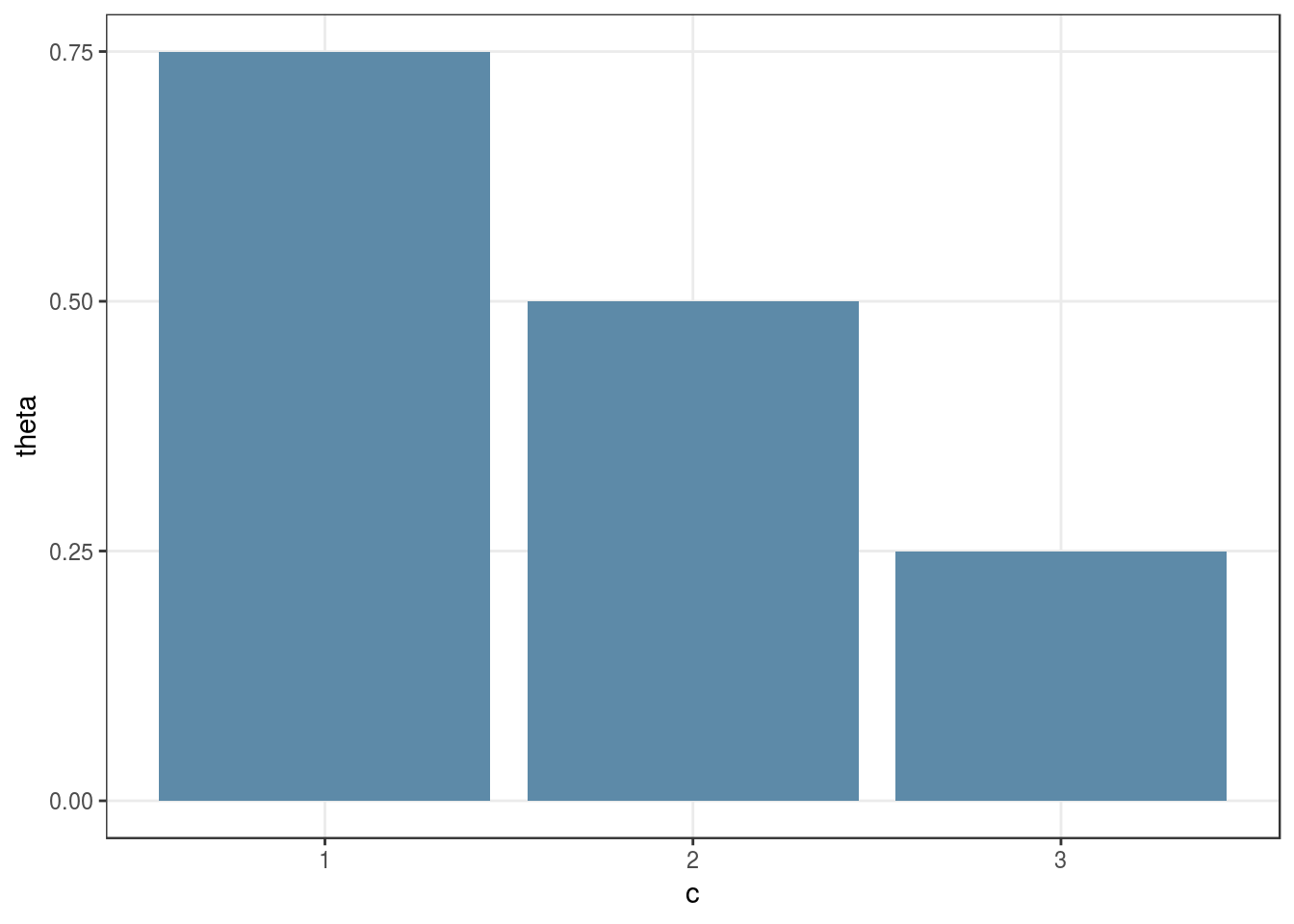
And here’s a plot of the likelihood:
tibble(
  c = 1:3,
  theta = c(0.75, 0.50, 0.25)
) %>%
  ggplot() +
  geom_col(
    aes(c, theta),
    fill = theme_color
  ) +
  scale_x_continuous(breaks = 1:3,
                     minor_breaks = NULL) +
  scale_y_continuous(breaks = seq(0, 1, 0.25),
                     minor_breaks = NULL) +
  theme_bw()
Note that the likelihood function is discrete because the hidden quantity is the coin’s identity rather than the probability of heads (we know \(\theta_c\) for all \(c\)). In the classic coin tossing problem, our knowledge is reversed. We are given the outcome of \(n\) coin tosses and want to infer \(\theta\) for a single coin. The resulting likelihood function in that case is continuous, as we vary \(\theta\) to figure out which values were more likely to generate the observed quantity \(x\). Even though in both problems we’re talking about coins, they end up being quite different!
We can visually see that the maximum likelihood estimate for the coin’s identity in this case is \(C_{ML} = \text{argmax}(0.75) = 1\).
The posterior with a uniform prior
The goal of Bayesian inference is to compute the posterior, i.e. the probability of the parameters given the data. In this case that means computing:
\[ Pr(C = c \mid X = x) \]
We can do this via Bayes rule:
\[ Pr(C = c \mid X = x) = \frac{Pr(X = x \mid C = c) \times Pr(C = c)}{Pr(X = x)} \]
where:
- \(Pr(X = x \mid C = c)\) is the probability of the data given the parameters, a.k.a the likelihood
- \(Pr(C = c)\) is the probability of the parameters before seeing the data (prior belief), a.k.a the prior
- \(Pr(X = x)\) is the probability of the data, a.k.a the marginal probability of the data.
By the law of total probability, the denominator can be re-written as:
\[ Pr(X = x) = \sum_{y} Pr(X = x \mid C = y) \times Pr(C = y) \]
where we use \(y\) instead of \(c\) to denote that the sum is over all possible values of \(C\) and avoid confusion between the two variables.
Because the likelihood is not a valid probability distribution, it’s the job of the denominator to make sure that the posterior is one. That is why the denominator is often interpreted as a normalising constant (it can also be interpreted as a probability distribution). We can therefore write that the posterior is proportional to the likelihood times the prior2:
\[ Pr(C = c \mid X = x) \propto \Pr(X = x \mid C = c) \times Pr(C = c) \]
A single coin toss
Continuing with the example of a single coin toss \(x = 1\), we now assume that the 3 coins are equally likely to be picked from the bag. This is equivalent to choosing the discrete uniform distribution for our prior:
\[ Pr(C = c) = 1/3 \]
This is clearly a valid probability distribution as \(\sum_{c=1}^{3} Pr(C=c) = 1\). We usually want to use valid probability distributions for our priors to ensure that the posterior is also one3.
Now that we understand how to calculate the likelihood and prior, we introduce Baye’s Box which help us to compute the denominator (normalising constant), and hence the posterior, by hand:
| Parameter | Likelihood | Prior | Likelihood \(\times\) Prior | Posterior |
|---|---|---|---|---|
| C | \(Pr(X = 1 \mid C =c)\) | \(Pr(C = c)\) | \(Pr(X = 1 \mid C = c) \times Pr(C=c)\) | \(Pr(C = c \mid X = 1)\) |
| 1 | 3/4 = 0.75 | 1/3 = 0.333 | 3/12 = 0.2500 | 3/6 = 0.500 |
| 2 | 2/4 = 0.50 | 1/3 = 0.333 | 2/12 = 0.1667 | 2/6 = 0.333 |
| 3 | 1/4 = 0.25 | 1/3 = 0.333 | 1/12 = 0.0833 | 1/6 = 0.167 |
| Total | 1.5 | 1 | 6/12 = 0.5 | 1 |
Looking at the table we can confirm that:
- The Likelihood is not a valid probability distribution (I know I’m repeating this ad nauseum but repetition is at the core of learning)
- The Prior is a valid (discrete) probability distribution
- The Posterior is a valid (discrete) probability distribution, i.e. \(\sum_{c=1}^{3} Pr(C =c \mid X = 1) = 1\)
- The denominator is calculated as the sum of the likelihood times the prior over all possible values parameter values, and its job is to normalise the posterior (the normalising constant).
Multiple coin tosses
For \(n\) tosses of the same coin, we adapt the random variable \(X\) to represent the number of times we record heads in \(n\) coin tosses: \(X \in \{0,1,\ldots,n\}\). For a given sample of \(x\) heads, we can calculate the likelihood using the probability mass function for the binomial distribution, which models the outcome of \(n\) independent Bernoulli trials (only two possible outcomes per trial):
\[ \begin{equation} L(C = c \mid x) = Pr(X = x \mid C = c) = \binom{n}{x} \theta_{c}^{x}(1-\theta_{c})^{n-x} \tag{1} \end{equation} \] Therefore, for two coin tosses and \(X = 2\), we have:
x     <- 2 # number of heads
c     <- 1:3
theta <-  c(0.75, 0.50, 0.25)

lik   <- dbinom(x = 2, size = 2, p = theta) # likelihood
prior <- rep(1/3, 3)
num   <- lik * prior # numerator
denom <- sum(num) # denominator
post <- num/denom # posterior| Parameter | Likelihood | Prior | Likelihood \(\times\) Prior | Posterior |
|---|---|---|---|---|
| C | \(Pr(X = 2 \mid C =c)\) | \(Pr(C = c)\) | \(Pr(X = 2 \mid C = c) \times Pr(C=c)\) | \(Pr(C = c \mid X = 2)\) |
| 1 | 0.5625 | 0.333 | 0.1875 | 0.6429 |
| 2 | 0.2500 | 0.333 | 0.0833 | 0.2857 |
| 3 | 0.0625 | 0.333 | 0.0208 | 0.0714 |
| Total | 0.875 | 1 | 0.292 | 1 |
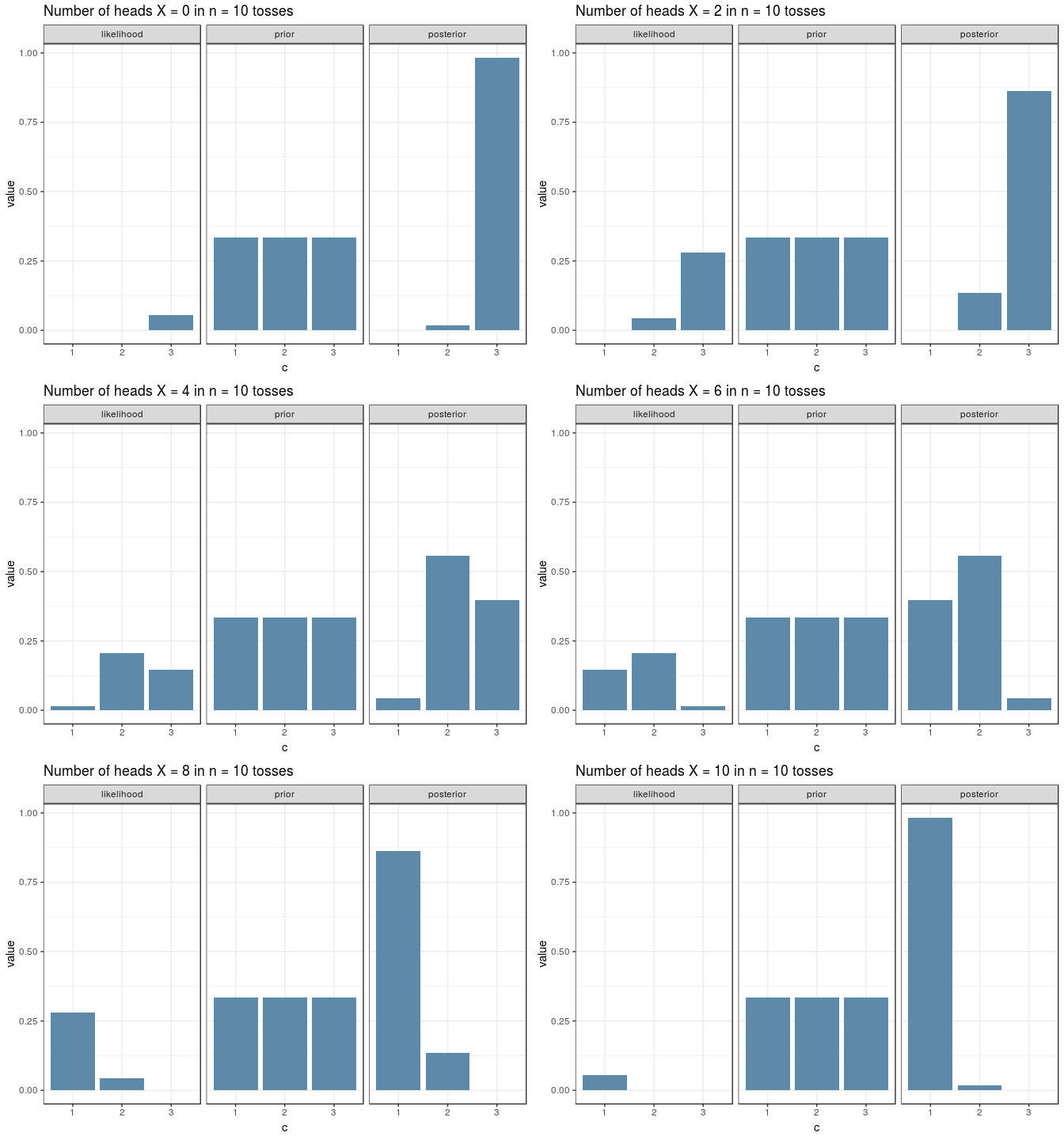
And here’s a visualisation for an experiment with \(n=10\) just because the ggplot + gganimate combo is awesome. Note how the shape of the posterior resembles the one of the likelihood, given a uniform prior:

An informative prior
In the previous section we introduced an uninformative prior for \(C\). Despite flat priors being often interpreted as uninformative, its use is discouraged by prominent Bayesian statisticians. Instead, weakly informative priors should often guide an objective analysis (let the data speak for itself). The discussion about the subjectivity and objectivity of Bayesian priors is a long and contentious one. Please refer to the book and works of Gelman, among others, for more details.
Here, the book provides an example of an informative prior, which places much belief on the coin’s identity being biased towards tails:
\[ \begin{align} Pr(C = 1) &= 1/20\\ Pr(C = 2) &= 5/20\\ Pr(C = 3) &= 14/20 \end{align} \]
We now use Baye’s box again to compute the marginal and posterior distributions, and understand how changing the prior affects the posterior and the resulting inference:
x     <- 2 # number of heads
c     <- 1:3
theta <- c(0.75, 0.50, 0.25)

lik   <- dbinom(x = 2, size = 2, p = theta) # likelihood
prior <- c(1/20, 5/20, 14/20)
num   <- lik * prior # numerator
denom <- sum(num) # denominator
post <- num/denom # posterior| Parameter | Likelihood | Prior | Likelihood \(\times\) Prior | Posterior |
|---|---|---|---|---|
| C | \(Pr(X = 2 \mid C =c)\) | \(Pr(C = c)\) | \(Pr(X = 2 \mid C = c) \times Pr(C=c)\) | \(Pr(C = c \mid X = 2)\) |
| 1 | 0.5625 | 0.05 | 0.0281 | 0.209 |
| 2 | 0.2500 | 0.25 | 0.0625 | 0.465 |
| 3 | 0.0625 | 0.70 | 0.0437 | 0.326 |
| Total | 0.875 | 1 | 0.134 | 1 |
We can now calculate summary statistics of our posterior distribution:
# Posterior Mean
sum(post * c)
## [1] 2.116279# Maximum a posterior (MAP) estimate for c
which.max(post)## [1] 2# Maximum likelihood estimate
which.max(lik)## [1] 1The posterior mean in this instance is very close to \(c=2\), so if we had to make a decision about the coin’s identity that would be relatively straightforward. In one sense, it is useful because it tells us how close the expected value is to each parameter value. However, we can imagine that, with a different dataset, the resulting mean could lie between parameter values (e.g. 1.5). In that instance, making a decision about the coin’s identity would be a lot more difficult using the mean. The MAP (Maximum A Posteriori) or maximum likelihood estimate, on the other hand, always give a straight answer. In this case, they disagree due to the effect of the prior: \(C_{MAP}=2\), \(C_{ML}=3\).
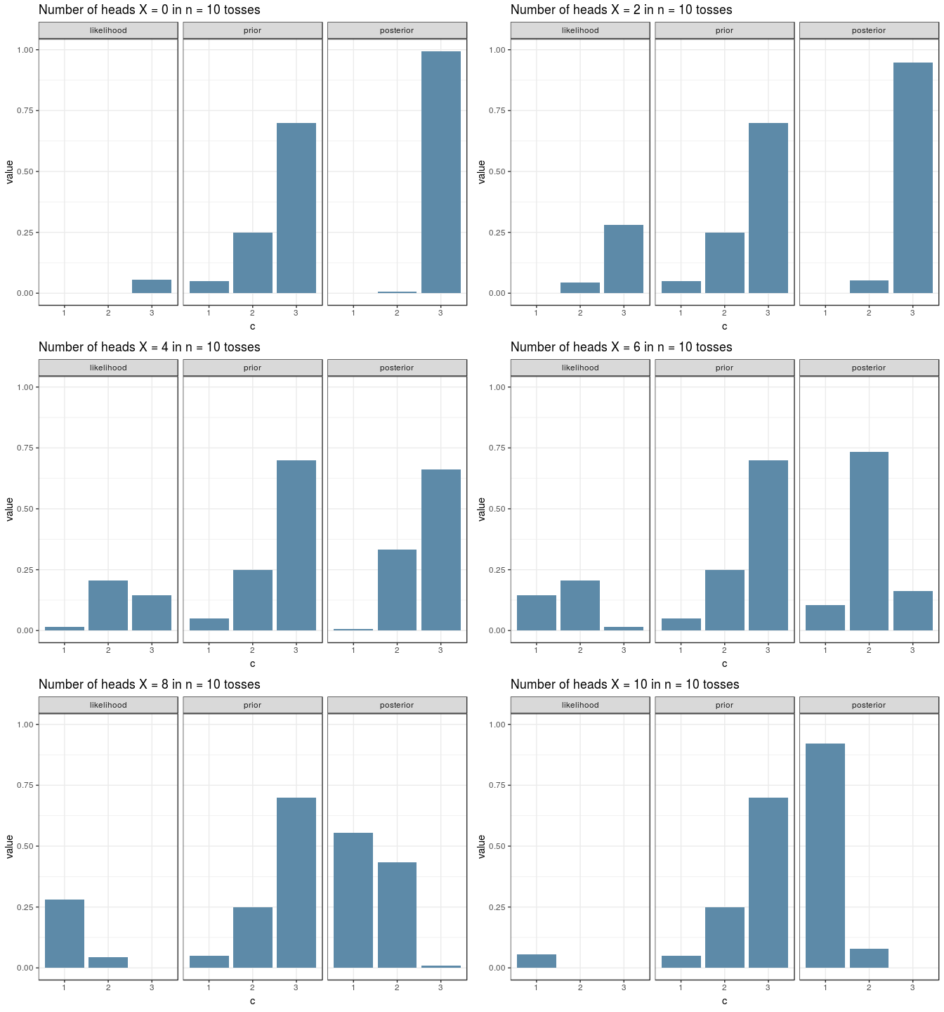
And here’s the same visualisation as before, for an experiment with \(n=10\), for the new prior. Note how the shapes of the posterior and likelihood are now different.

The Posterior Predictive Distribution
Consider the single coin toss example again: \(n =1, x = 1\). If we where to flip the coin a second time, how does first observing heads change our belief about the outcome of the second flip? Are we more, less or equally confident about obtaining heads in the second flip?
We can answer this question via the posterior predictive distribution. With the uniform prior on \(C\), the posterior predictive distribution, in this case, can be obtained using the expression:
\[ Pr(\tilde{X} \mid X = 1) = \sum_{c=1}^{3} Pr(\tilde{X} \mid C) \times Pr(C \mid X = 1) \]
where \(\tilde{X}\) is the result of a new coin flip. But where does this expression come from?
- \(Pr(\tilde{X} \mid C)\) is the likelihood of new data \(\tilde{X} \in \{0,1\}\) given the coin’s identity \(C\). Guess what? It’s the same expression that we used before: the binomial distribution!
\[ \begin{align} & Pr(\tilde{X} = 1 \mid C = 1) = \theta_1 \\ & Pr(\tilde{X} = 1 \mid C = 2) = \theta_2 \\ & \ldots \\ & Pr(\tilde{X} = 0 \mid C = 3) = 1 - \theta_3 \end{align} \]
- \(Pr(C \mid X = 1)\) is the posterior that we’ve also calculated above:
\[ \begin{align} & Pr(C = 1 \mid X = 1) = 3/6\\ & Pr(C = 2 \mid X = 1) = 2/6\\ & Pr(C = 3 \mid X = 1) = 1/6 \end{align} \]
You can interpret the posterior predictive distribution as the average of the probability of a single coin toss (likelihood) weighted by the posterior. For instance, if we want to find the probability of a new coin toss resulting heads, then we average \(\theta_c\) over all values of \(c\), weighted by how likely we think that each parameter is to occur given the previously observed outcome. It is the posterior that provides the weights for each parameter!
In general, to find the posterior predictive distribution, you sample a parameter value from the posterior, feed that into your likelihood function, repeat the process many times and 💥 you have a probability distribution capable of predicting new data based on the old data!
x     <- 1 # number of heads
c     <- 1:3
theta <- c(0.75, 0.50, 0.25)
post  <- c(3/6, 2/6, 1/6)

new_x <- c(0,1)
lik_new_x <- matrix(c(1-theta, theta),
                    nrow = 2,
                    byrow = TRUE)

post.pred <- lik_new_x %*% matrix(post, nrow = 3)

rownames(post.pred) <- c("Pr(new_X = 0 | X = 1) = ", "Pr(new_X = 1 | X = 1) = ")
colnames(post.pred) <- ""

post.pred
##
## Pr(new_X = 0 | X = 1) = 0.4166667
## Pr(new_X = 1 | X = 1) = 0.5833333So, if we had to guess the next coin flip, based on the first outcome being heads (and our model: prior + likelihood), we’d probably put our money on heads.
Model evaluation is about checking how well it can reproduce the data generating process. Maybe our likelihood function is not adequate. Maybe our choice of prior is poor. The posterior predictive distribution is one way to address these questions. But there is a lot more to model evaluation than just computing the posterior predictive distribution (in most instances we can only approximate it by sampling from the posterior). In short, how good your model is depends on its ability to generate extreme values present in the data. Read more about this topic on chapter 10 of the book.
In the meantime, happy modelling ∩ coding!
see chapter 4 of the book for more details↩
see chapter 6 and 7 of Ben Lambert’s book for more details.↩
please refer to chapters 5 the book for a more in depth discussion on the validity of priors↩